Parallel processing has revolutionized the way we approach computation-intensive tasks, allowing us to fully utilize the capabilities of modern multi-core processors and drastically reduce the time it takes to perform complex calculations. In both Python and R, parallel processing opens up a world of possibilities for developers and data scientists alike. In this post we will work through some practical examples to uncover how these languages facilitate parallel execution to tackle real-world challenges. Whether you are handling big data, running simulations, or optimising algorithms, understanding the parallel processing capabilities of either Python or R is key to unlocking new levels of speed and efficiency in your computational endeavors.
The concept of parallel processing in Python or R is not new and there is plenty of material out there on this topic. So why another post on parallel processing? Firstly, for the fun of it, I juxtapose Python and R solutions which is not common. Second, most examples that I managed to come across on parallel processing were a little too elementary for my taste which left me wondering how to get more advanced applications it to work for me. While my examples don’t claim superiority, they aim to provide a smoother transition from rudimentary to more advanced computations.
To illustrate how to get started with parallel processing and to highlight the efficiency gains that are up for grabs we will consider a basic, non-parallel application. We will then migrate this example to a parallel infrastructure and measure the difference. After this, we will attempt some more advanced computations as we try to move to statistical applications.
A non-parallel approach
As a approach, consider the sleep functionality, time.sleep() in Python and base::Sys.sleep() in R. Both functions suspend code execution for a specified number of seconds. For clarity, let’s write a function called wait() that takes in an integer parameter called seconds. When called, this function will wait for the amount of seconds specified.
Assume that we need to call this function multiple times and, well, wait each time we call it. To action this requirement, we position the wait() function in a timed loop and have it print a message every time it is done waiting. In our case, we will call wait() an arbitrary amount times, say , ten. We will wait two seconds each time and measure how long it took at the end. As with any for loop, these function calls occur sequentially.
# load timing libraryimport time# create a wait() functiondef wait(seconds): time.sleep(seconds)# run wait() in a timed looptic = time.perf_counter()for i inrange(10): wait(seconds=2)print(f'Done waiting for thing {i+1}')toc = time.perf_counter()print(f'Duration: {toc - tic} seconds')
Done waiting for thing 1
Done waiting for thing 2
Done waiting for thing 3
Done waiting for thing 4
Done waiting for thing 5
Done waiting for thing 6
Done waiting for thing 7
Done waiting for thing 8
Done waiting for thing 9
Done waiting for thing 10
Duration: 20.014614800000345 seconds
# load timing packagelibrary(tictoc)# create a wait() functionwait <-function(seconds) {Sys.sleep(seconds)} # run wait() in a timed looptictoc::tic()for (i inc(1:10)){wait(seconds =2)print(paste("Done waiting for thing", i))}tictoc::toc()
[1] "Done waiting for thing 1"
[1] "Done waiting for thing 2"
[1] "Done waiting for thing 3"
[1] "Done waiting for thing 4"
[1] "Done waiting for thing 5"
[1] "Done waiting for thing 6"
[1] "Done waiting for thing 7"
[1] "Done waiting for thing 8"
[1] "Done waiting for thing 9"
[1] "Done waiting for thing 10"
20.27 sec elapsed
Calling wait() ten times took approximately twenty seconds. Suppose we need to hurry up and wait, but we still need to wait ten times. What if we could just wait all ten times at the same time? Enter parallel processing. In short, parallel processing splits a computational process across multiple CPUs or multiple cores of a CPU in order to decrease runtime (we will limit our discussion to CPU-bound processes here, which are more suited to the type of computations we want to pursue).
Make it parallel
There are a few options available for parallel computing in Python and R, but we will stick to the multiprocessing module and doParallel. Depending on the processing power avaiable to us, we should be able to reduce our runtime significantly. It is useful to check how many CPU cores are available to us especially if we want to control the number of cores the computation should be allowed to use. multiprocessing.cpu_count() and parallel::detectCores() are available to determine this in Python and R respectively. These functions return integers as output, and we can simply subtract the number of cores we want to preserve before telling multiprocessing or doParallel how many cores to use. With this in mind, let’s hurry up and wait(). We can examine each implementation separately below:
If you are using an interactive interpreter like Ipython on Windows, using certain components from the multiprocessing library can be tricky. Here is an excerpt from the multprocssing module’s documentation:
CautionNote:
Functionality within this package requires that the __main__ module be importable by the children. This is covered in Programming guidelines however it is worth pointing out here. This means that some examples, such as the multiprocessing.pool.Pool examples will not work in the interactive interpreter.
Without getting technical, the consequence is that if our wait() function is defined in the same script used to run wait() in parallel, the Python will just hang forever. The solution to getting around this is to create a separate script in the same directory as the script you are working from. This script should contain the function that we want to run in parallel. Let’s create a defs.py file and place our functions in there.
Create script defs.py in the same directory as your working script, and include the wait() function.
def wait(things, seconds=2):""" Toy function for parallel processing example. """ time.sleep(seconds)returnf'Done waiting for thing {things +1}'
Import defs.py into your working script as a module with import wait:
import defs # import my script as moduleimport timeimport multiprocessing as mpcores = mp.cpu_count()tic = time.perf_counter()if__name__=='__main__':with mp.Pool(processes=cores) as pool:for i in pool.map(defs.wait, range(10)):print(i)toc = time.perf_counter()print(f'Cores available at runtime: {cores}')print(f'Duration: {toc - tic} seconds')
Done waiting for thing 1
Done waiting for thing 2
Done waiting for thing 3
Done waiting for thing 4
Done waiting for thing 5
Done waiting for thing 6
Done waiting for thing 7
Done waiting for thing 8
Done waiting for thing 9
Done waiting for thing 10
Cores available at runtime: 24
Duration: 2.193319900005008 seconds
Note
If you are running python in another way (e.g. from the command line) it should be fine to source everything in the same script.
Note
You will notice that I follow a package::function() convention for in all the R code. I don’t code like this on a regular basis, but rather include package calls here to indicate which package each function comes from in case you are unfamiliar a particular function.
library(doParallel) # also loads foreach and parallelcores <- parallel::detectCores()cluster <- parallel::makeCluster(cores)doParallel::registerDoParallel(cluster)tictoc::tic()foreach::foreach(i =c(1:10)) %dopar% {wait(seconds=2)print(paste("Done waiting for thing", i))}tictoc::toc() print(paste("Cores available at runtime:", cores))parallel::stopCluster(cluster)
[[1]]
[1] "Done waiting for thing 1"

[[2]]
[1] "Done waiting for thing 2"

[[3]]
[1] "Done waiting for thing 3"

[[4]]
[1] "Done waiting for thing 4"

[[5]]
[1] "Done waiting for thing 5"

[[6]]
[1] "Done waiting for thing 6"

[[7]]
[1] "Done waiting for thing 7"

[[8]]
[1] "Done waiting for thing 8"

[[9]]
[1] "Done waiting for thing 9"

[[10]]
[1] "Done waiting for thing 10"

2.12 sec elapsed
Cores available at runtime: 24
The results show that we waited 10 times, at the same time, which means we waited for a total of just over 2 seconds. This arithmetic works because we had more than 10 cores available at runtime, but ended up with ten processes using ten cores. If the number of cores were less than the number of times we called wait() the total runtime would have been longer. Let’s try a slightly more complicated example: importing data from files, transforming the data and then writing them to file again as a csv.
A File I/O Application
We use S&P 500 tick data from kibot. See this note for more information on this data and how to get it. Simply download the data, put it in a directory of your choice and read it in as below. Some basic data exploration reveals that we are dealing more than ten million rows of data.
import pandas as pdimport numpy as np# set display options to show more digitspd.options.display.float_format ='{:7,.2f}'.format# read in the data from where my data is storeddf = pd.read_csv('../data/IVE_tickbidask.txt', header=None, names=['day', 'time', 'price', 'bid', 'ask', 'vol'], engine='c', dtype={'day':str, 'time':str, 'price':np.float64, 'bid':np.float64, 'ask':np.float64,'vol':np.int64 })# parse a datetime columndf['datetime'] = pd.to_datetime(df['day'] + df['time'], format='%m/%d/%Y%H:%M:%S')df = df.set_index('datetime').drop(columns=['day', 'time'])df.head()
library(data.table)library(tidyverse)library(skimr)# read in the data from where my data is storeddf <- data.table::fread("../data/IVE_tickbidask.txt", header=FALSE, colClasses=c("character","character","numeric","numeric","numeric","numeric"))names(df) <-c("day", "time", "price", "bid", "ask", "vol")# parse a datetime columndf <- df |> tibble::as_tibble() |> tidyr::unite("datetime", c(day, time), remove =TRUE, sep =" ") |> dplyr::mutate(datetime =mdy_hms(datetime))head(df)
We are going to apply a set of arbitrary transformations to the data and write the results back to disk. We leave out a non-parallel example (I challenge you to test the time difference). While the mathematical transformations used here have no practical value, we accomplish two things. First, we illustrate how to apply a set of mathematical computations, albeit basic, to the same data set and store the results - all in parallel. Second, we manage to iterate in parallel over varying sets of inputs (function parameters in our case).
We write a function that takes in a dataframe and applies some arithmetic to all the numeric columns. The calculation starts by taking the natural log or square root, depending on the type parameter. The function then subtracts an arbitrary number, multiplies it with an arbitrary number and then raise it to an arbitrary power. The result is then written straight to disk in csv format.
For such large data sets we would usually write to parquet, but csv is a more common format and the slower writing time to csv serves to help highlight the gains in parallel (if you took the time to try a non-parallel version of this example). When it comes to csv, data.table::fwrite() is significantly faster than pd.to_csv().
def transform(df, subtract, multiply, power, type, out_name):""" A function to apply mathematical transformations to the numerical columns of a dataframe """iftype=='log': df.apply(lambda x: ((np.log(x) - subtract)*multiply)**power if np.issubdtype(x.dtype,np.number) else x ).to_csv( out_name )eliftype=='sqrt': df.apply(lambda x: ((np.sqrt(x) - subtract)*multiply)**power if np.issubdtype(x.dtype,np.number) else x ).to_csv( out_name )print(f'Done writing {out_name}')
Using starmap() allows us to map over a list of multiple varying parameters.
import osimport timeimport multiprocessing as mpimport defs # import my script as a modulefrom functools import partial# collate parameter arguments in a list of tuplesargs = [(0, 0.652, 2, 'log', 'data/parallel_processing/tickdata_tr.csv'), (-1, 0.2, 3, 'log', 'data/parallel_processing/tickdata_tr1.csv'), (9, 0.463, 2, 'sqrt', 'data/parallel_processing/tickdata_tr2.csv'), (20, 0.8, 3, 'sqrt', 'data/parallel_processing/tickdata_tr3.csv')]tic = time.perf_counter()if__name__=='__main__':with mp.Pool(4) as p:# starmap() will return a list which is empty in our case because we # are not assigning the results to a variable, but writing them to the # hard drive instead. It need not work this way. p.starmap(partial(defs.transform, df), args)toc = time.perf_counter()print(f'Duration: {toc - tic} seconds')# verify that the files have written to the correct folderos.listdir('data/parallel_processing')
To iterate over varying parameters, we don’t do anything fancy (e.g. purrr::map()). For the R example, simply iterating through a nested list in a parallel loop does the job. Keep in mind this is just one approach meant to illustrate the usefulness of parallel processing.
library(doParallel)library(tictoc)transform <-function(df, subtract, multiply, power, type, out_name) {if (type =="log") { df <- dplyr::mutate(df, dplyr::across(price:vol, ~ (log(.x) - subtract*multiply)^power)) |> data.table::fwrite(out_name) } elseif (type =="sqrt") { df <- dplyr::mutate(df, dplyr::across(price:vol, ~ (sqrt(.x) - subtract*multiply)^power)) |> data.table::fwrite(out_name) }return(paste("Done writing", out_name))}# collate arguments into a nested listargs <-list(list(subtract =0, multiply =0.652, power =2, type ='log', out_name ='data/parallel_processing/tickdata_tr.csv'),list(subtract =-1, multiply =0.2, power =3, type ='log', out_name ='data/parallel_processing/tickdata_tr1.csv'),list(subtract =9, multiply =0.463, power =2, type ='sqrt', out_name ='data/parallel_processing/tickdata_tr2.csv'),list(subtract =20, multiply =0.8, power =3, type ='sqrt', out_name ='data/parallel_processing/tickdata_tr3.csv'))cluster <- parallel::makeCluster(4)doParallel::registerDoParallel(cluster)tictoc::tic()foreach::foreach(i =c(1:length(args))) %dopar% { p = args[[i]]transform(df, p$subtract, p$multiply, p$power, p$type, p$out_name)}tictoc::toc() parallel::stopCluster(cluster)# verify that the files have written to the correct folderlist.files('data/parallel_processing')
For our final example let’s take a stab at constructing an equally weighted portfolio of tech stocks and then calculate a Value-at-Risk (VaR) measure. To keep the focus on parallel processing, we leave out the theory on VaR and simply calculate. We also leave out a non-parallel example and head straight to the parallel implementation.
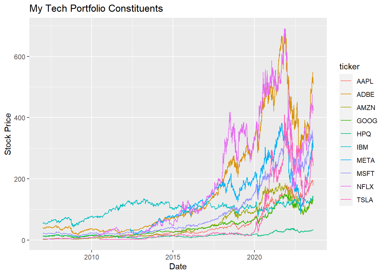
Let’s calculate the VaR measure using a monte carlo simulation. We will implement with parallel processing based on historical returns. First, we collect stock prices from Yahoo! Finance for ten major tech companies that we want to invest in and include in to My Tech Portfolio.
import yfinance as yfimport pandas as pdimport plotly.express as pximport numpy as nptickers = ["AAPL","GOOG","TSLA","IBM","NFLX","ADBE","META","AMZN","MSFT","HPQ"]df = yf.download(tickers, '2007-01-01')['Adj Close']df_return = df.pct_change().melt(ignore_index=False, value_name ='return').reset_index(names='date')df = df.melt(ignore_index=False).reset_index(names='date').merge(df_return, how='left', on=['date', 'variable'])px.line(df, x='date', y='value', color='variable', title='My Tech Portfolio Constituents', labels={'indexed_return':'Indexed Return', 'date':'Date'})
[                       0%%                      ]
[**********            20%%                      ]  2 of 10 completed
[**************        30%%                      ]  3 of 10 completed
[*******************   40%%                      ]  4 of 10 completed
[**********************50%%                      ]  5 of 10 completed
[**********************60%%***                   ]  6 of 10 completed
[**********************70%%********              ]  7 of 10 completed
[**********************80%%************          ]  8 of 10 completed
[**********************90%%*****************     ]  9 of 10 completed
[*********************100%%**********************]  10 of 10 completed
library(tidyverse)library(quantmod)library(doParallel)# library(plotly)# Create a vector containing the official stock symbolstickers <-c("AAPL","GOOG","TSLA","IBM","NFLX","ADBE","META","AMZN","MSFT","HPQ")# Set up parallel clustercores <- parallel::detectCores()cluster <- parallel::makeCluster(cores)doParallel::registerDoParallel(cluster)# this parallel loop outputs to a list of tibble dataframesextract <- foreach::foreach(i =c(1:length(tickers))) %dopar% {# package calls also need to be explicit in child processes data <- quantmod::getSymbols(tickers[i], auto.assign=FALSE) |> tsbox::ts_tbl() |> tidyr::separate(id, c("ticker", "price_type")) |> dplyr::rename(date = time)} parallel::stopCluster(cluster)# parse list to a single dataframestock_data <- dplyr::bind_rows(extract)# extract only the adjusted closing price and calculate a simple returnadjusted_price <- stock_data |> dplyr::filter(price_type =="Adjusted") |> dplyr::select(-price_type)plot <- ggplot2::ggplot(adjusted_price, ggplot2::aes(x = date, y = value, colour = ticker)) + ggplot2::geom_line() + ggplot2::labs(title ="My Tech Portfolio Constituents",x ="Date",y ="Stock Price" )plot
# plotly::ggplotly(plot)
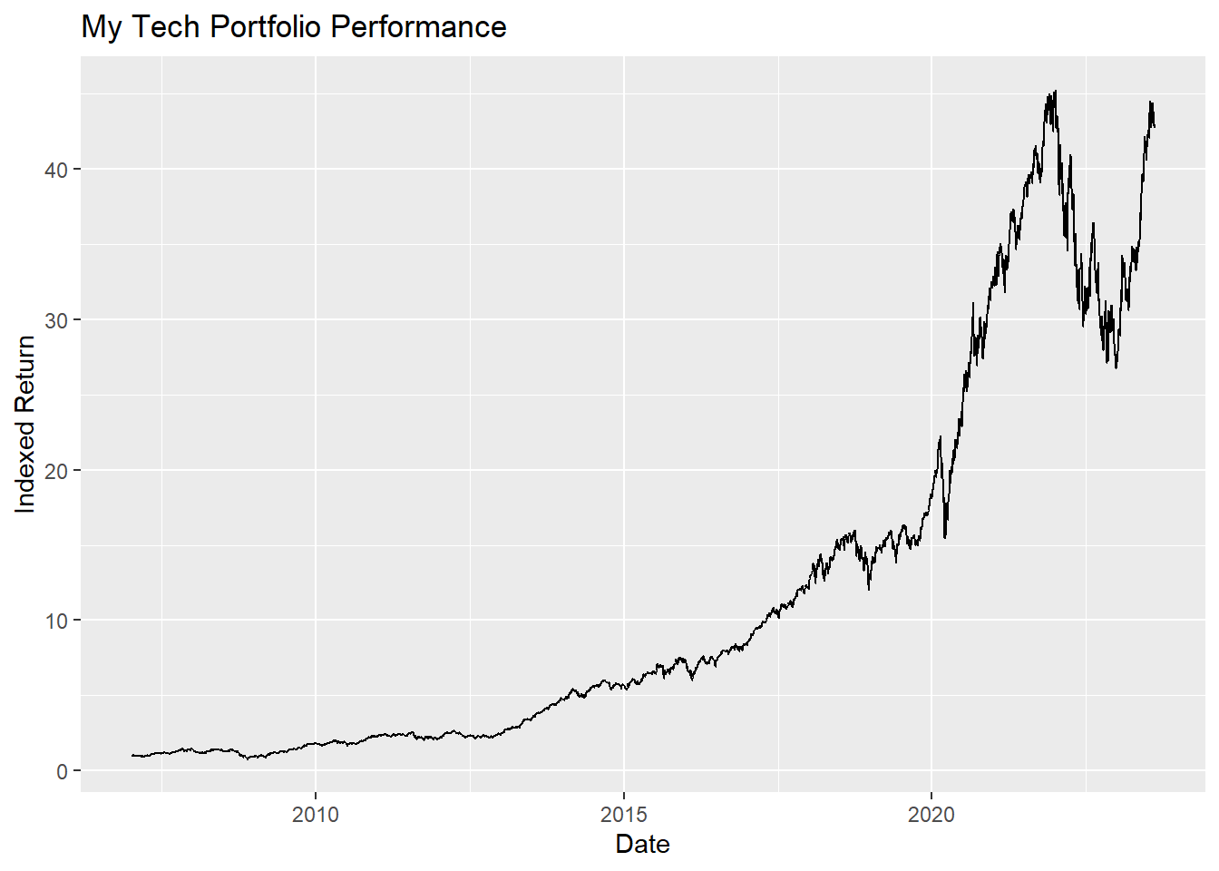
I like to calculate an indexed return and then chart that to see performance over time. Essentially, this indexed return shows us how well our investment would have done if we invested $1 in the My Tech Portfolio at the start of the period in question and held it to the end of that period.
Having constructed our portfolio, we can move on to simulating and calculating the VaR. It is common practice to choose a 95% confidence interval (\(\alpha = 0.05\)). We will sample from the historical returns distribution 10 0000 times, and then forecast the VaR over the next 7 days.
def single_simulation(horizon, returns):""" A single instance of a simulation that can be run multiple times. """ simulated_returns = np.random.choice(returns, size=horizon, replace=True) simulated_portfolio_value = np.prod(1+ simulated_returns) # Assuming simple returnsreturn simulated_portfolio_value
import multiprocessing as mpimport defsalpha =0.05n_simulations =10000horizon =7args = [(horizon, df_portfolio['portfolio_ret'].to_numpy())] * n_simulationsif__name__=="__main__": p = mp.Pool(mp.cpu_count()) # Use all available CPU cores# Run simulations in parallel portfolio_values = p.starmap(defs.single_simulation, args) p.close() p.join()sorted_values = np.sort(portfolio_values)var_index =int(n_simulations * alpha)historical_var =-sorted_values[var_index] # Multiply by -1 to get positive VaRprint(f"Historical VaR ({alpha *100:.2f}%): {historical_var:.4f}")
Historical VaR (5.00%): -0.9395
# Set parametersalpha <-0.05# Confidence level for VaRn_simulations <-10000# Number of simulationshorizon <-7# Forecast horizon (7-day VaR)# Function for a single Monte Carlo simulationsingle_simulation <-function(returns) {# Simulate portfolio returns for the specified horizon simulated_returns <- base::sample(returns, size = horizon, replace =TRUE)# Calculate the portfolio value for the horizon using the simulated returns simulated_portfolio_value <- base::prod(1+ simulated_returns) # Assuming simple returnsreturn(simulated_portfolio_value)}cores <- parallel::detectCores()cluster <- parallel::makeCluster(cores)doParallel::registerDoParallel(cluster)# Parallelise the Monte Carlo simulationsportfolio_values <- foreach::foreach(i =1:n_simulations, .combine ="c") %dopar% {single_simulation(portfolio$portfolio_ret)}parallel::stopCluster(cluster)# Calculate historical VaRsorted_values <- base::sort(portfolio_values)var_index <- base::round(n_simulations * alpha)historical_var <--sorted_values[var_index] # Multiply by -1 to get positive VaRpaste0("Historical VaR (", alpha *100, "%) for the portfolio is: ", historical_var)
[1] "Historical VaR (5%) for the portfolio is: -0.936797488799702"
The result means that, according to this metric, 5% of the time over the next 7 days we can expect to have a loss in My Tech Portfolio of at least -94%. To recap, we split our data collection process across multiple cores (for R. Python is fast enough non-parallel) and proceeded to calculate an equally weighted portfolio of tech stocks. We used the distribution of historical returns in a monte carlo simulation to sample returns and forecast returns. We were able to split the simulation over multiple cores into individual jobs to speed up the process.
Conclusion
Parallel processing is a very useful tool to keep around for any sort of computation or process. There are many, many more different types of use cases and applications than what I’ve illustrated here. Hopefully these examples help you nudge a little closer to real world application with out feeling too lost.
Some reading for the bath
The list of links here cover important things I did not touch on in this post and also provide some additional applications and methods. Some of these articles sit behind a paywall.